Week1 & Week2:
-
Gradient descent inference including cost function definition and derivative is on slices.
-
feature scaling and mean normalization is helping speed up gradient descent.
\[x_i = \frac{x_i-\mu_i}{max-min}\]
- Normal Equation: Gradient descent gives one way of minimizing J. Let’s discuss a second way of doing so, this time performing the minimization explicitly and without resorting to an iterative algorithm. In the “Normal Equation” method, we will minimize J by explicitly taking its derivatives with respect to the θj ’s, and setting them to zero. This allows us to find the optimum theta without iteration. The normal equation formula is given below:
\[\theta = (X^TX)^{-1}X^Ty\]
Gradient descent has time complexity \(O(kn^2)\); Normal Equation is \(O(n^3)\), in which n is the number of features. In practice, when n exceeds 10,000 it might be a good time to go from a normal solution to an iterative process.
If \(X^TX\) is noninvertible, the common causes might be having :
- Redundant features, where two features are very closely related (i.e. they are linearly dependent)
- Too many features (e.g. m ≤ n). In this case, delete some features or use “regularization” (to be explained in a later lesson).
Solutions to the above problems include deleting a feature that is linearly dependent with another or deleting one or more features when there are too many features
- Gradient descent learning rate \(\alpha\)
- If \(alpha\) is too small: slow convergence.
- If \(alpha\) is too large: may not decrease on every iteration and thus may not converge.
Week 3: Classification
We cannot use the same cost function that we use for linear regression because the Logistic Function will cause the output to be wavy, causing many local optima. In other words, it will not be a convex function.
Instead, our cost function for logistic regression looks like:
\(Cost(h_\theta, y) = -log(h_\theta(x)) if y = 1\) \(Cost(h_\theta, y) = -log(1 - h_\theta(x)) if y = 0\)
- Since this cost function leads to:
- \(Cost(h_\theta, y) = 0\) if \(h_\theta(x) = y\)
- \(Cost(h_\theta, y)\) -> \(\infty\) if y = 0 and \(h_\theta(x) -> 1\)
- \(Cost(h_\theta, y)\) -> \(\infty\) if y = 1 and \(h_\theta(x) -> 0\)
- This cost function is convex.
Put together:
\(Cost(h_\theta, y) = -ylog(h_\theta(x)) - (1-y)log(1-h_\theta(x))\)
There are other alternative to minimize \(J(\theta)\) other than gradient descent, no detailed introduction to them.
Underfitting, or high bias, is when the form of our hypothesis function h maps poorly to the trend of the data. It is usually caused by a function that is too simple or uses too few features. At the other extreme, overfitting, or high variance, is caused by a hypothesis function that fits the available data but does not generalize well to predict new data
This terminology is applied to both linear and logistic regression. There are two main options to address the issue of overfitting:
1) Reduce the number of features:
- Manually select which features to keep.
- Use a model selection algorithm.
2) Regularization
- Keep all the features, but reduce the magnitude of parameters \(\theta_j\)
- Regularization works well when we have a lot of slightly useful features.
linear regression
We could also regularize all of our theta parameters in a single summation as:
\[min_\theta \frac{1}{2m} \sum^m_{i=1}(h_\theta(x^{i}) - y^{i})^2 + \lambda\sum^{n}_{j=1}\theta^2_j\]
The λ, or lambda, is the regularization parameter. It determines how much the costs of our theta parameters are inflated.
Using the above cost function with the extra summation, we can smooth the output of our hypothesis function to reduce overfitting. If lambda is chosen to be too large, it may smooth out the function too much and cause underfitting.
The gradient descent iterations & Normal Equation become: https://www.coursera.org/learn/machine-learning/supplement/pKAsc/regularized-linear-regression
Regularized Logistic Regression
\[J(\theta) = -\frac{1}{m}\sum_{i=1}^{m}[y^ilog(h_\theta (x^i)) + (1-y^i)log(1-h_\theta (x^i)] + \frac{\lambda}{2m}\sum_{j=1}^n \theta ^2_j\]
https://www.coursera.org/learn/machine-learning/supplement/v51eg/regularized-logistic-regression
Week4 & Week5 Neuron Network
-
For neural networks, the cost function would be on https://www.coursera.org/learn/machine-learning/supplement/afqGa/cost-function
-
The inference of back-propagation is listed here: https://www.cs.swarthmore.edu/~meeden/cs81/s10/BackPropDeriv.pdf
- Random Initialization:
- Zero initialization: After each update, parameters corresponding to inputs going into each of hidden units are identical.
- Key will be init values shouldn’t be the identical.
- Gradient checking code: https://www.coursera.org/learn/machine-learning/supplement/fqeMw/gradient-checking
Week 6 Evaluating a learning algo.
One way to break down our dataset into the three sets is:
- Training set: 60%
- Cross validation set: 20%
- Test set: 20%
Why is cross validation needed?
- Model selection: Without cross validation dataset, given multiple model candidates, we pick a model by selecting the model with the smallest test error on the testing datasetset with parameters trained on related training data. However, we cannot tell how good the model’s generalization is by using test data sets again since the selected model has been fit to the test dataset (Will lead to over-optimized). Thus, we add cross-validation dataset which will be used to select model, test data set will be used to estimate the model’s generalization error.
One way to break down our dataset into the three sets is:
- Training set: 60%
- Cross validation set: 20%
- Test set: 20%
We can now calculate three separate error values for the three different sets using the following method:
- Optimize the parameters in Θ using the training set for each polynomial degree.
- Find the polynomial degree d with the least error using the cross validation set.
- Estimate the generalization error using the test set with \(J_{test}(\Theta^{(d)})\), (d = theta from polynomial with lower error); This way, the degree of the polynomial d has not been trained using the test set.
How to choose the regularization lambda?
- https://www.coursera.org/learn/machine-learning/supplement/JPJJj/regularization-and-bias-variance
- https://d3c33hcgiwev3.cloudfront.net/b0cf48c6b7bc9f194310e6bc90dec220_Lecture10.pdf?Expires=1605312000&Signature=a7tVdZrfdSZe4eb3Z87OXpw4OGf96q~p3kyUkBRSgh1ebO8rCzl98Pc4vnkMkapbg5jcVxbUbMaq9a44W9wgikDm1wlCMwl0YtJohKBVsfx8twPciPlMs5~xi84T4h6ZHL-Ih8v3MuGCl8kfi8XrXq2XGM0Bejzc6jPmAEO7t5k&Key-Pair-Id=APKAJLTNE6QMUY6HBC5A
Change Hyper Parameter:
Our decision process can be broken down as follows:
- Getting more training examples: Fixes high variance
- Trying smaller sets of features: Fixes high variance
- Adding features: Fixes high bias
- Adding polynomial features: Fixes high bias
- Decreasing λ: Fixes high bias
- Increasing λ: Fixes high variance.
Error Analysis The recommended approach to solving machine learning problems is to:
- Start with a simple algorithm, implement it quickly, and test it early on your cross validation data.
- Plot learning curves to decide if more data, more features, etc. are likely to help.
- Manually examine the errors on examples in the cross validation set and try to spot a trend where most of the errors were made.
For example, assume that we have 500 emails and our algorithm misclassifies a 100 of them. We could manually analyze the 100 emails and categorize them based on what type of emails they are. We could then try to come up with new cues and features that would help us classify these 100 emails correctly. Hence, if most of our misclassified emails are those which try to steal passwords, then we could find some features that are particular to those emails and add them to our model. We could also see how classifying each word according to
Use evidence to find cues instead of gut feeling
https://www.coursera.org/learn/machine-learning/lecture/x62iE/error-analysis is interesting.
Precision and Recall
Why Precision / Recall
- To deal with skewed data.
How to remember True/False Positive/Negative False/True are from a prediction perspective. The predicted Positive/Negative is true or false?
Precision: Of all patients where we predicted y = 1, what fraction actually has cancer? True positive / (True positive + False positive) Recall: Of all patients that actually have cancer, what fraction did we correctly detect as having cancer? True positive / (False negative + True positive)
We usually use 1 to represent the rare cases.
Tradeoff between precision and recall
\(F_1\) score: \(2*\frac{PR}{P+R}\). Both recall and precision should large, or F score will be small.
We could use F score to pick threshold for classifier instead of always using 0.5
Week7: SVM (Large Margin, try to split the data as big a margin as possible)
\[min_\theta \sum_{i=1}^m cost_1(\theta^Tx^{i}) + (1-y^{i}) cost_0(\theta^Tx^{i}) + \lambda\sum_{i=0}^n \theta_j^2\]
https://d3c33hcgiwev3.cloudfront.net/246c2a4e4c249f94c895f607ea1e6407_Lecture12.pdf?Expires=1605571200&Signature=HLTXP1YKth~4F~T8ibWgd0pRL0jvUyw-GQdsIdBpjkqg9Es95IMmtg91NFchg1ei0C3try2XCxt8LBhUIng-Wjkh6fSpeQGDO9~o1FMDvTppQKwxTYiLDrSE4qO-4iuXUYZX5cYFU5wLdGDyBGIDEkomVMBpZfyWJdLlmGm5xtk&Key-Pair-Id=APKAJLTNE6QMUY6HBC5A
Kernels:
Why Kernels: to deal with Non-linear Dicision Boundary.
Predict y = 1 if \(\theta_0 + \theta_1x_1 + \theta_2x_2 + \theta_3 x_1x_2 + \theta_4 x_1^2 + … >= 0 \)
My understanding of kernels is instead of using the absolute value of training data, we use the relative location relations between a given training set and the remainings to classify data.
Bias & variance tradeoffs could be adjusted by \(\theta\) and C
Use SVM software package (e.g. liblinear, libsvm, …) to solve for parameters \(\theta\).
Need to specify:
- Choice of parameter C.
- Choice of kernel (similarity function):
E.g. No kernel (“linear kernel”): Predict “y = 1” if \(\theta ^ T x >= 0\), when features number is large but training set is small (to avoid high dimension overfit)
Gaussian kernel:
\(f_i = exp(-\frac{||x-l^i||^2}{2\delta^2})\), where \(l^i = x^i\). Need to choose \(\delta^2\)
Note: Do perform feature scaling before using the Gaussian kernel.
Not all similarity functions \(similarity(x, l)\) make valid kernels. (Need to satisfy technical condition called “Mercer’s Theorem” to make sure SVM packages’ optimizations run correctly, and do not diverge).
Many off-the-shelf kernels available:
- Polynomial kernel: \(k(x, l) = (x^Tl)^2\)
- More esoteric: String kernel, chi-square kernel, histogram intersection kernel, …
Logistic regression vs. SVMs
n = number of features(x belongs to \(R^{n+1}\)), m= number of training examples.
- If n is large (relative to m):
- Use logistic regression, or SVM without a kernel (“linear kernel”)
- If n is small(1-1000), m is intermediate (10-10,000): Use SVM with Gaussian kernel.
- If n is small, m is large (m = 50,000+) Create/add more features, then use logistic regression or SVM without a kernel. SVM is too slow
Neural network likely to work well for most of these settings, but may be slower to train.
Week8: Unsupervised Learning: Introduction:
- Market segmentation
- Social network analysis
- Organize computing clusters
- Astronomical data analysis
K mean clustering algo:
Move centroids interactively. Random init centroids.
Randomly init K cluster centroids \(\mu_1, \mu_2, … \mu_k\) Repeat { for i = 1 to m Cluster assignment for k = 1 to K move centroid }
K-means for non-separated clusters
Local optima: Solutions: Random initialization
For i=1 to 100 {
Randomly initialize K-means.

Run K-means. Get \\(c^{(1)}, ..., c^{(m)}, \mu_1, ..., \mu_K\\)

Compute cost function (distortion)
    \\(J(c^{(1)}), ... c^{(m)}, \mu_1, ... \mu_K) \\)
}
How to choose cluster number of K.
Elbow method:
- Obtain cost function and try a different number of K, pick the K followed by a flatlands.
- Evaluate the K number based on metrics for how well it performs for the later purpose.
Dimensionality Reduction (PCA):
- Data Compression
- Speed up training
- Data Visualization
Try to find a surface so as to minimize projection error.
Data preprocessing: mean & scaling.
\(Sigma=\frac{1}{m}\sum_{i=1}{m}(x^{i})(x^{i})^T\)
\([U, S, V] = U(:, 1:k);\)
\(z = Ureduce’ * x\)
Choosing k (number of principal components)
Average squared projection error: \(\frac{1}{m} \sum_{i=1}{m} (x^{i}-x_approx^{i}) ^2\) Total variation in the data: \(\frac{1}{m} \ sum_{i=1}{m} (x^i) ^2\)
Typically, choose k to be smallest value so that: Average error / Total variation <= 0.01
99% of variance is retained.
Or use S in [U, S, V] = svd(Sigma)
\(1-\frac{\sum_{i=1}{k}S_{ii}}{\sum_{i=1}{n}S_{ii}} <= 0.01\)
Week 9
Anormaly detection
- Fraud detection
- Manufacturing
- Monitoring computers in a data centers
How to calculate it:
- \(x_1, x_2…\) are features of a inference record.
- \(P(x) = p(x_1, \mu, \theta^2)p(x_2; \mu, \theta^2)..\)
- \(\prod{j=1}{n} p(x_j; \mu_j, \theta_j^2)\)
How to find \(\epsilon\)
- Assume we have some labeled data, of anomalous and non-anamalous examples (y=0 if normal, y=1 if anomalous) Cross validation set + Test set.
Training set: 6000 good engines, no anomalous. CV: 2000 good engines(y=0), 10 anomalous(y=1) Test: 2000 good engines(y=0), 10 anomalous(y=1)
Try different \(\epsilon\) on cross validation set (finding new features will be also on cross validation set), and pick the one maximize F-score.
Possible evaluation metrics:
- F1
- F-score
Anormaly Detection vs. Supervised Learning
Anomaly detection:
- Very small number of positive example (y=1) (0-20 is common)
- Large number of negative (y=1) example.
- Many different types of anomalies, Hard for any algo to learn from positive examples what the anomalies look like.
- Future anomalies may look nothing like any of the anomalous examples we’ve seen so far.
Supervised learning:
- Large number of positive and negative examples.
- Enough positive examples for algo to get a sense of what positive examples are like, future positive examples likely to be similar to ones in training set.
What features to use
- Plot features histogram, Non-gaussian features should be somehow mathematically converted to Gaussian distribution using like log, cube, square, ^1/2, etc.
- Error analysis to find potential new features.
- Choose features that might take on unusually large or small values in the event of an anomaly.
Multivariate Gaussian distribution: Catch Correlation among multiple vars.
- Original model: 1) Manully create feature to capture anomalies where \(x_1, x_2\) take unusual combinations of values (\(x_3=\frac{x_1}{x_2}\)). 2) Computationallly cheaper. 3) OK even if m(training set size) is mall
- Multitivariate Gaussian: 1) Automatically captures correlations between features. 2) computationally more expensive 3) Must have m>n (m>=10n) or else \(\sum\) is non-invertible.
Predicting Movie Ratings.
Content-based recommender systems:
Problem formulation:
\(r(i,j)=1\) if user j has rated movie i(0 otherwise) \(y^{(i, j)}\) = rating by user j on movie i (if defined)
\(\theta^j = \) parameter vector for user j \(x^{i} = \) parameter vector for user i For user j, movie i, predicted rating: \((\theta^{j})^T(x^{i})\)
To learn \(\theta^{(j)}\)
\[ min_\theta^j \frac{1}{2m^j} \sum_{i:r(i, j)=1}(\theta^j)^T(x^i)-y^{(i, j)})^2 + \frac{\lambda}{2m^j}\sum_{k=1}^{n}(\theta_k^j)^2 \]
Collaborative Filtering:
Feature Learning: An algo taking stuff to learn itself what features to use.
- Initialize \(x^1, x^2… x^n, \theta^1, \theta^2… \theta^n\) to small random values.
- Minimize \(J(x^1, … x^n, \theta^1… \theta^n)\) using gradient descent.
- For a user with parameters \(\theta\) and a move with (learned feature x), predict a star rating of \(\theta^Tx\)
Finding related movies (distance among data)
Mean Normalization: To remove \(\theta = 0\) for unknown user.
Week 10
Learning with Large Datasets:
Assume m = 100,000,000
- Try small dataset like 1000 records and plot learning curve to see if it is high-variance.
- Stochastic gradient descent
- Original Batch Gradient descent will go through all training datasets to calculate one iteration of \(\theta\). Stochastic instead, will adjust the \(\theta\) according to a single training record
- Mini-Batch Gradient Descent:
- Mini-batch gradient descent: Rather than using single example as in Stochastic, use b examples in each iteration. The reason why it is faster than stochastic gradient descent is mini-batch could be optimised by “vectorize computation”
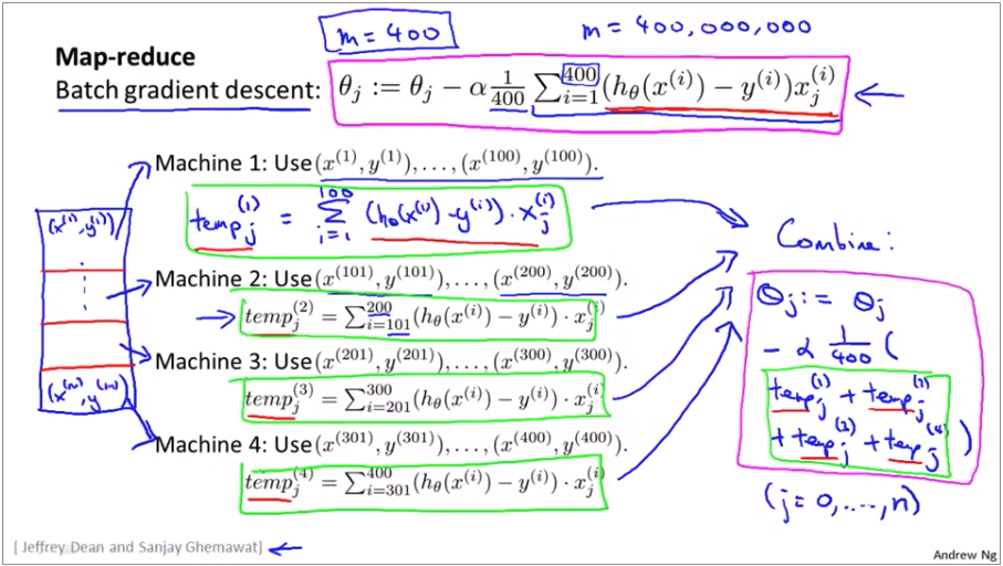
Batch gradient descent:
- Plot \(J_{train}(\theta)\) as a function of the number of iterations of gradient descent.
Stochastic gradient descent:
- \(cost(\theta, (x^i, y^i)) = 1/2(h_\theta(x^i)-y^i)^2\)
- During learning, compute \(cost(\theta, (x^i, y^i))\) before updating \(\theta\) using \((x^i, y^i)\).
- Every 1000 iterations(say), plot cost\((\theta, x^i, y^i)\) averaged over the last 1000 examples processed by algorithm.
Learning rate \(\alpha\) is typically held constant. Can slowly decrease over time if we want \(\theta\) to converge (\(\alpha = \frac{const1}{iterationNumber+const2}\))
Online Learning Shipping service website where user comes, specifies origin and destination, you offer to ship their package for some asking price, and users sometimes chosse to use your shipping service (y=1), sometimes not (y=0).
Feature x capture properties of user, of origin/destination and asking price, we want to learn \(p(y=1|x;\theta)\) to optimize price.
Logistic regression:
Repeat forever {
Get (x, y) corresponding to user.

Update \\(\theta\)) using (x, y):

    \theta_j = \theta_j - \alpha(h_\theta(x)-y)*x_j (j=0, ..., n)
}
Can adapt to change user preference.
Product search (learning to search)
User searches for Android phone 1080p camera.

Have 100 phones in store, will return 10 results.

x = features of phone, how many words in user query match.

name of phones, how many words in query match description of phone, etc.

Learn \\(p(y=1|x; \theta)\\)
Other examples: Choosing special offers to show user; customized selection of news articles; product recommendation.
MapReduce: Many learning algo can be expressed as computing sums of functions over the training set.
Week 11 ML Application
Discussion on getting more data
- Make sure you have a low bias classifier before expending the effort. (Plot learning curves). E.g. Keep increasing the number of features/number of hidden units in neural network until you have a low bias classifier.
- How much work would it be to get 10x as much data as we currrently have?
Ceiling Analysis:: What part of the pipeline to work on next: What part of the pipeline should you spend the most time trying to improve?
- Overall system accuary 72%
- If text detection is 100% correct, the overall system will be 89%.
- Character segmentation …, the overall system will be 90%.
- Character recognition …, the overall system will be 100%.
So text detection could be increased and have a potential 17% improvement impact. Character recognition could have a potential impact of 10% improvement.